Introduction to fastCNV - Visium HD data
fastCNV_HD.RmdContext
fastCNV is a package to detect the putative Copy Number
Variations (CNVs) in single cell (scRNAseq) data or Spatial
Transcriptomics (ST) data. It also plots the computed CNVs.
In this vignette you will learn how to run this package on Visium HD seurat object. fastCNV runs on Seurat5.
Warning : Visium HD samples are very RAM demanding and the session may crash if not enough RAM is available. We recommend running this vignette in a server.
Load packages
To get the example data used in this vignette, you’ll need to install
and load the fastCNVdata package.
remotes::install_github("must-bioinfo/fastCNV")
remotes::install_github("must-bioinfo/fastCNVdata")Check annotation
You can load a separate annotation file for your dataset. It’s usefull to have annotated spots for the analysis.
# Import the annotation file corresponding to your sample. For 10X ST data you can annotate your spots with LoupeBrowser. The example data already has the annotations in it.
annotation_file <- read.csv("/path/to/your/annotations/for/VisiumHD.csv")

HDBreast[["annots_8um"]] <- annotation_file$Annotations
You can take a look at which annotations are present in your objects, in order to select the labels of the cells that will be used as reference.
unique(HDBreast[["annots_8um"]])
#>                       annots_8um
#> s_016um_00107_00066-1
#> s_008um_00269_00526-1    NoTumor
#> s_008um_00260_00253-1      Tumor
fastCNV will use by default the 16µm assay, so if your annotations are done on the 8µm resolution you will need to run this function before running fastCNV on the 16µm assay. This function maps the annotations from the 8µm resolution to the 16µm resolution.
HDBreast <- annotations8umTo16um(HDBreast, referenceVar = "annots_8um")
#> [1] "New annotation column (new referenceVar) is named : projected_annots_8um."
Now the 16um spots also have the annotations given to the 8um spots. The projected annotations are in the meta data “projected_annots_8um”. This will be the referenceVar we will use from now on.
You can check if the projected annotations are correct by doing
SpatialDimPlot(HDBreast, group.by = "projected_annots_8um")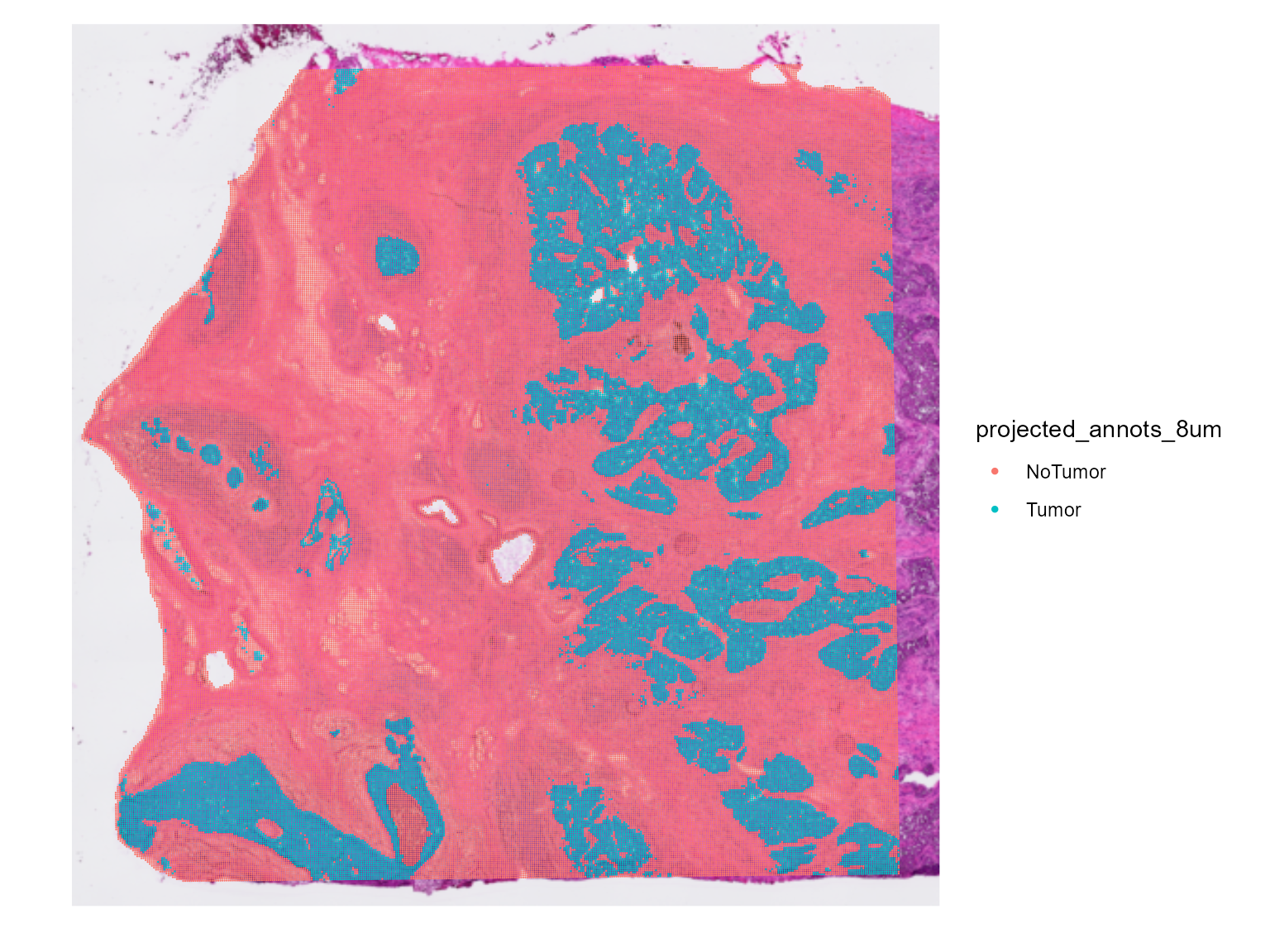
Run fastCNV
During this step, fastCNV_10XHD() will use:
CNVAnalysis: computes the CNV. If you have annotations for your Seurat object, you can add the parametersreferenceVarandreferenceLabel.CNVPerChromosome: to compute the CNV per chromosome arm, and store it in the metadata of the Seurat object. This part offastCNV()can be skipped by turninggetCNVPerChromosometoFALSE.CNVCluster: OPTIONAL - performs hierarchical clustering on a genomic score matrix extracted from a Seurat object. This may crash with large Visium HD samples. This function can be run later on.plotCNVResultsHD: to visualize the results (stored in the assays slot of the Seurat object). This function will also build a PNG or PDF file for each sample containing their corresponding CNV heatmap in the current working directory, which can be changed using thesavePathparameter.
We are going to run fastCNV() on our Visium HD object.
The reference should be the non-tumor spots, here “NoTumor”.
Warning : This can be very RAM demanding.
HDBreast <- fastCNV_10XHD(HDBreast, sampleName = "HDBreast", referenceVar = "projected_annots_8um", referenceLabel = "NoTumor", printPlot = TRUE)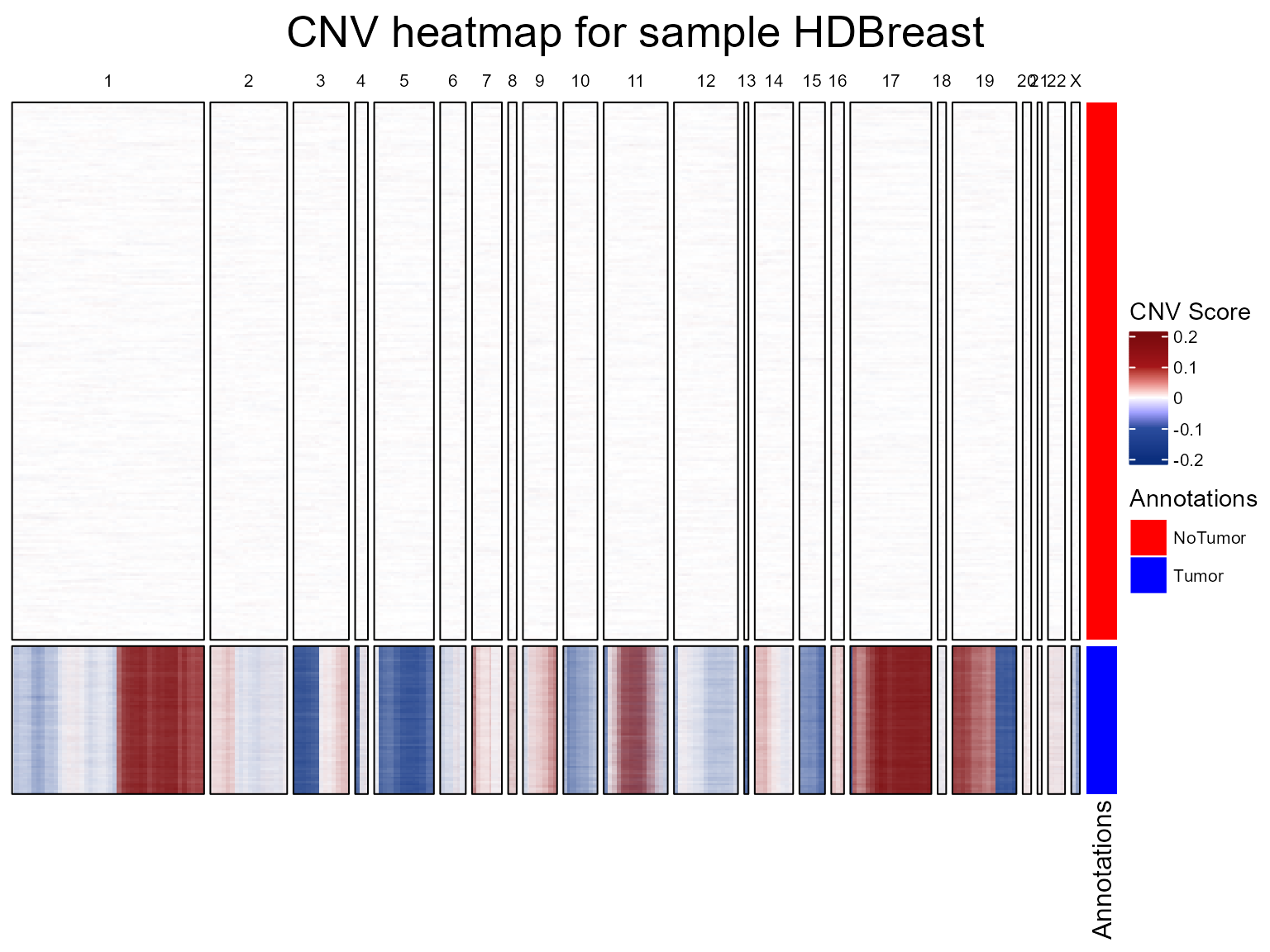
CNV fraction
fastCNV also computes a cnv_fraction for each
observation in the Seurat object. This can be directly plotted using
Seurat spatial plotting functions, as we’ll demonstrate on STColon1:
library(patchwork)
SpatialFeaturePlot(HDBreast, "cnv_fraction") | SpatialPlot(HDBreast, group.by = "projected_annots_8um")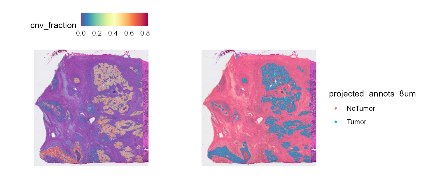
Here, we see some zones with higher CNV fractions than others. We can directly plot and test this:
library(ggplot2)
ggplot(FetchData(HDBreast, vars = c("projected_annots_8um", "cnv_fraction")),
       aes(projected_annots_8um, cnv_fraction, fill = projected_annots_8um)) +
  geom_boxplot() +
  theme(axis.text.x = element_text(angle = 45, vjust = 1, hjust = 1, color = "black"))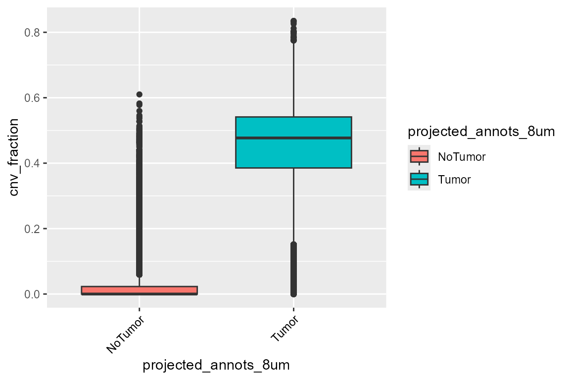
The tumor zone has a higher CNV fraction, which is coherent.
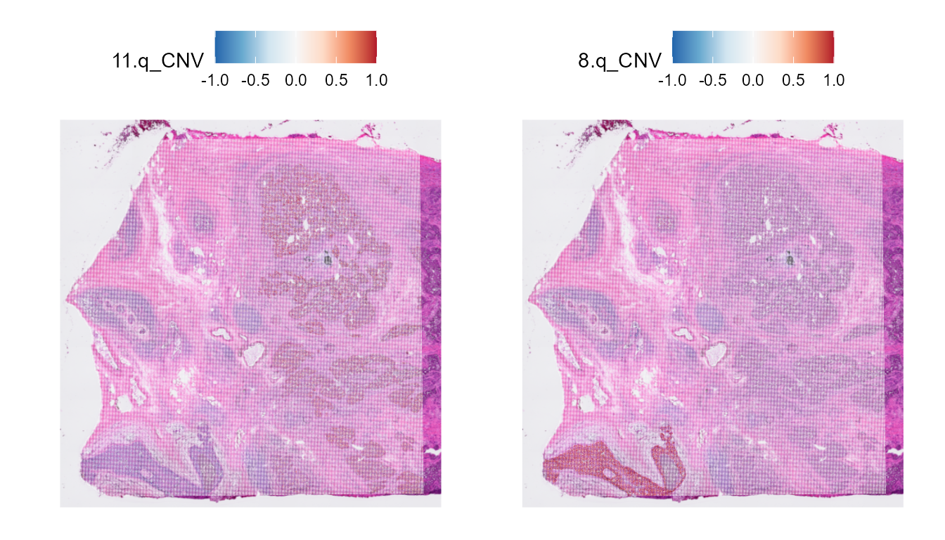
We can also plot the CNV per chromosome arm with the plotting functions from Seurat.
library(scales)

SpatialFeaturePlot(HDBreast, features = "11.q_CNV")  +
  scale_fill_distiller(palette = "RdBu", direction = -1, limits = c(-0.5, 0.5),
                       rescaler = function(x, to = c(0, 1), from = NULL) {
                         rescale_mid(x, to = to, mid = 0)
                       }) |
SpatialFeaturePlot(HDBreast, features = "8.q_CNV") +
  scale_fill_distiller(palette = "RdBu", direction = -1, limits = c(-0.5, 0.5),
                       rescaler = function(x, to = c(0, 1), from = NULL) {
                         rescale_mid(x, to = to, mid = 0)
                       })
CNV clusters
In addition to the CNV fraction, fastCNV also computes the CNV clusters. These can be plotted with the Seurat plotting functions.
SpatialDimPlot(HDBreast, group.by = "cnv_clusters") 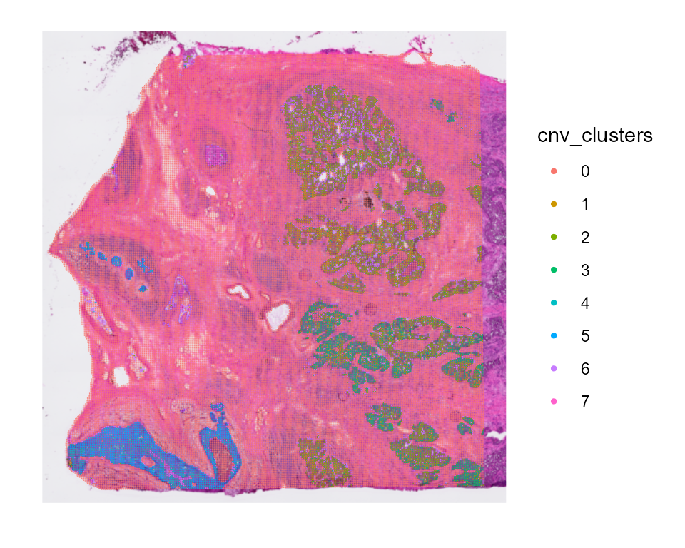 Here, we see many different CNV clusters with minimal variability. We
can compute the clusters only taking into account some annotations
(“tumor” here for example)
Here, we see many different CNV clusters with minimal variability. We
can compute the clusters only taking into account some annotations
(“tumor” here for example)
# To do the clustering with only certain annotations :
HDBreast <- CNVCluster(HDBreast, referenceVar = "projected_annots_8um",
                       cellTypesToCluster = "Tumor")

SpatialDimPlot(HDBreast, group.by = "cnv_clusters") 
Or merge the clusters with great correlation.
# To merge the clusters with high correlation
HDBreast <- mergeCNVClusters(HDBreast, mergeThreshold = 0.95) #adjust the thershold to your liking

SpatialDimPlot(HDBreast, group.by = "cnv_clusters") 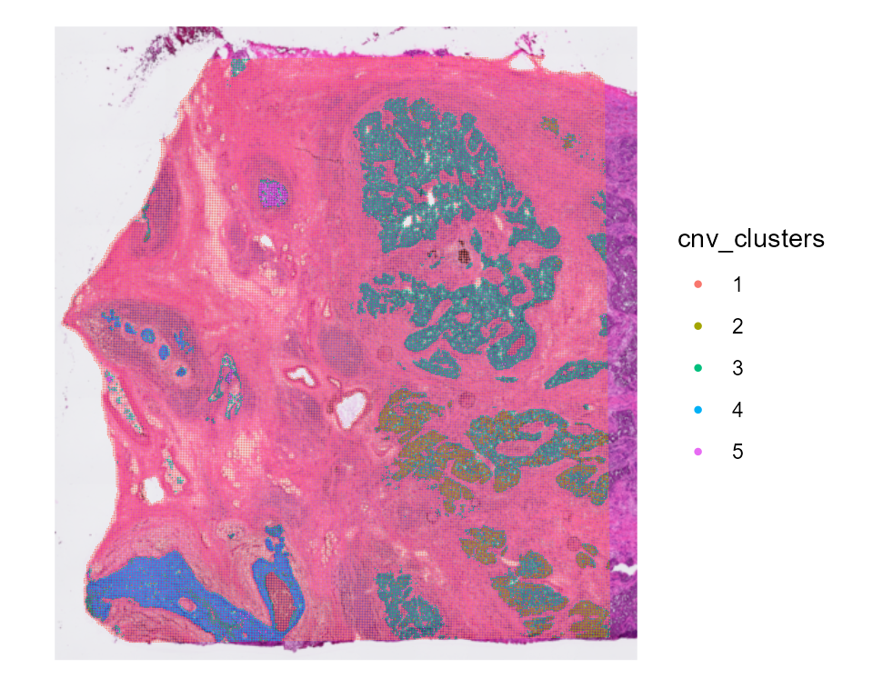
library(ggplot2)
library(SeuratObject)

HDBreast$cnv_clusters <- as.factor(HDBreast$cnv_clusters)
ggplot(FetchData(HDBreast, vars = c("cnv_clusters", "projected_annots_8um")), aes(projected_annots_8um, fill = cnv_clusters)) +
  geom_bar(position = "fill") +
  theme(axis.text.x = element_text(angle = 45, vjust = 1, hjust = 1, color = "black"))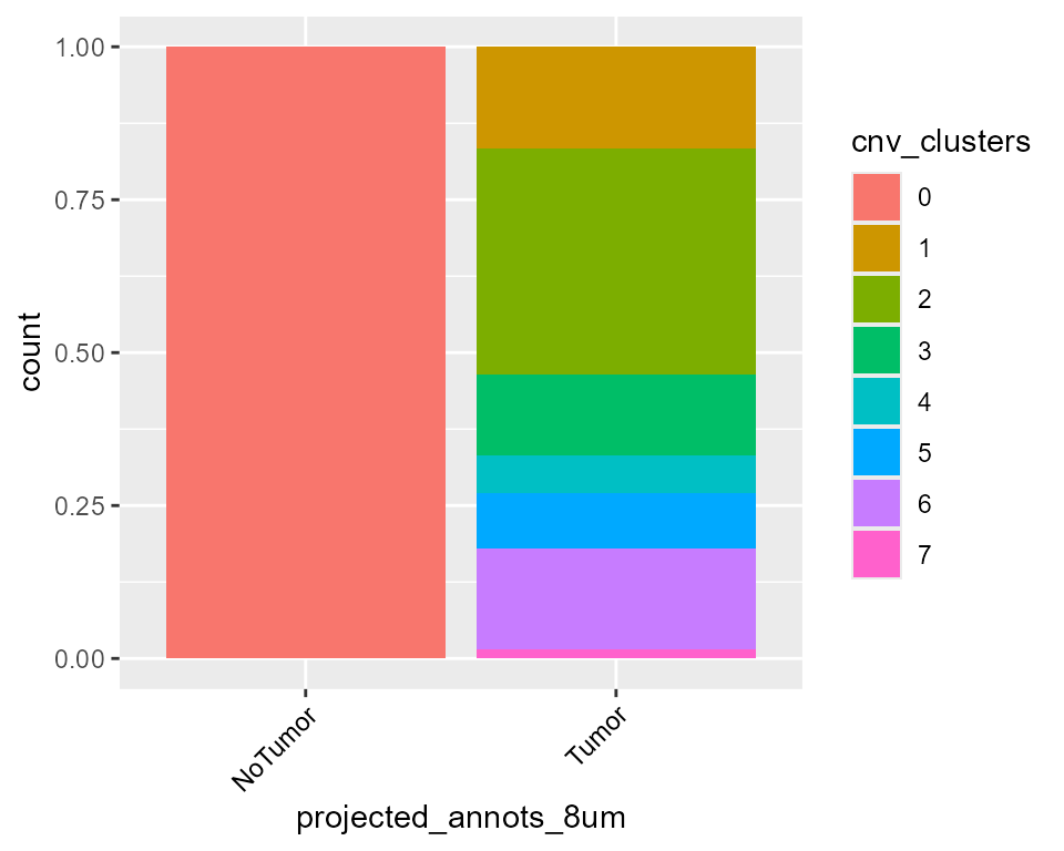
Once we have the desired clusters, we can do the CNV heatmap again to visualize the new clusters in it.
plotCNVResultsHD(HDBreast, referenceVar = "projected_annots_8um", printPlot = TRUE)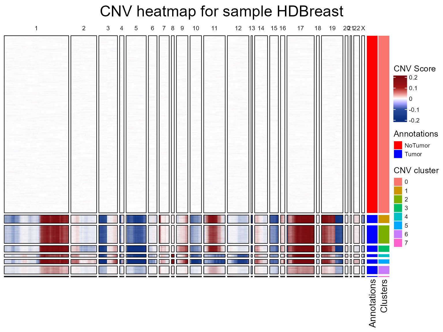
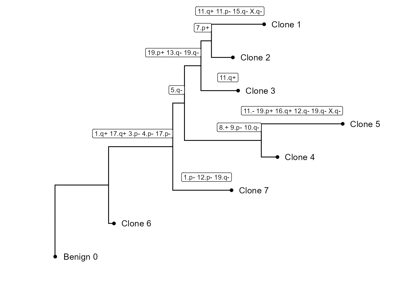
CNV tree
In this part of the vignette, we will show how to plot the CNV subclonality tree. CNV clusters are needed.
We build the tree, using CNVTree(). It contains the
following functions :
generateCNVClonesMatrixwill summarizefastCNV()’s results into a cluster/chromosome arm CNV matrix.buildCNVTree()will build the subclonality tree.annotateCNVTree()will annotate each cnv gain/loss in the tree.plotCNVTree()will output the tree.
tree_data <- CNVTree(HDBreast, values ="calls", cnv_thresh = 0.09, healthyClusters = "1")